ok so i have this homework in my Automatic controls class. i understand the concepts but for whatever reason i just cant get this problem to work out. i think its a problem with my modeling but im not sure. this is basically a system response problem. where i have some masses suspended by springs and dampers. the objective is to come out with the funtions for y1, and y2 (the displacements of the blocks where positive is downward) where i have 2 inputs u1 and u2 which will be constant forces. when i run it in matlab, im getting propagation rather than dampening, which is obviosly wrong. also since its multiple input (and linear) i have to treat this system as 2 single inputs working with the applied forces seperately and then adding them together in the end. the steps ive followed from my example are straight forward although it was only for a single input.
step 1: Identify input/output relationships
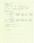
step 2: draw the FBD in the time domain
step 3: draw the FBD in the s domain (La Place transform)
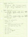
step 4: arrange the equations
step 5: put them in matrix format
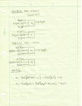
step 6: apply cramers rule to get the transfer funtions
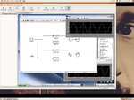
step 7: go into matlab for the simulation and plots of y1, y2
heres my work along with the matlab code:
step 1: Identify input/output relationships
step 2: draw the FBD in the time domain
step 3: draw the FBD in the s domain (La Place transform)
step 4: arrange the equations
step 5: put them in matrix format
step 6: apply cramers rule to get the transfer funtions
step 7: go into matlab for the simulation and plots of y1, y2
heres my work along with the matlab code:
Code:
% HW #2 - Problem #1

%Coefficients
m1=4;
m2=7;
k1=4.2;
k2=5.7;
b1=3.2;

% DEN(s)
aden=m1*m2;
bden=m1*b1+m2*b1;
cden=m1*k1+m2*k1;
dden=k1*b1+k2*b1;
eden=k1*k2;
den=[aden bden cden dden eden];

%NUM_11(s)
anum_11=m2;
bnum_11=b1;
cnum_11=k2;
num_11=[anum_11 bnum_11 cnum_11];

%NUM_21(s)
anum_21=b1;
bnum_21=0;
num_21=[anum_21 bnum_21];

%NUM_12(s)
anum_12=b1;
bnum_12=0;
num_12=[anum_12 bnum_12];

%NUM_22(s)
anum_22=m1;
bnum_22=b1;
cnum_22=k1;
num_22=[anum_22 bnum_22 cnum_22];

roots(den)
%Time vector
t=(0:0.05:60);
t=t';
%Introduce applied forces
for i=1:1201
    ua1(i)=2;
    ua2(i)=4;
end;
%Simulation using LSIM
sys1=tf(num_11,den);
sys2=tf(num_12,den);
sys3=tf(num_21,den);
sys4=tf(num_22,den);

y1_1=lsim(sys1,ua1,t);
y1_2=lsim(sys2,ua2,t);
y1=y1_1+y1_2;

y2_1=lsim(sys3,ua1,t);
y2_2=lsim(sys4,ua2,t);
y2=y2_1+y2_2;

%Plots y1 in green, y2 in red
subplot(211), plot(t,y1,'g');
subplot(212), plot(t,y2,'r');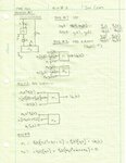

") i thought you had to sum after getting to the scope (which you cant) so i just summed them after the TF and then into the scope and it works
i thought you had to sum after getting to the scope (which you cant) so i just summed them after the TF and then into the scope and it works